Basic concept
Transformation affect the child nodes and as the name implies transforms them in various ways such as moving/rotating or scaling the child. Cascading transformations are used to apply a variety of transforms to a final child. Cascading is achieved by nesting statements e.g.
rotate([45,45,45])
  translate([10,20,30])
    cube(10);
Transformations can be applied to a group of child nodes by using '{' and '}' to enclose the subtree e.g.
translate([0,0,-5])
{
    cube(10);
    cylinder(r=5,h=10);
}
Transformations are written before the object they affect.
Imagine commands like translate, mirror and scale as verbs. Commands like color are like adjectives that describe the object.
Notice that there is no semicolon following transformation command.
Advanced concept
As OpenSCAD uses different libraries to implement capabilities this can introduce some inconsistencies to the F5 preview behaviour of transformations. Traditional transforms (translate, rotate, scale, mirror & multimatrix) are performed using OpenGL in preview, while other more advanced transforms, such as resize, perform a CGAL operation, behaving like a CSG operation affecting the underlying object, not just transforming it. In particular this can affect the display of modifier characters, specifically "#" and "%", where the highlight may not display intuitively, such as highlighting the pre-resized object, but highlighting the post-scaled object.
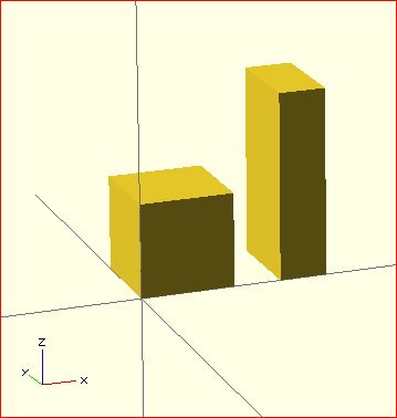
scale
Scales its child elements using the specified vector. The argument name is optional.
Usage Example:
scale(v = [x, y, z]) { ... }
cube(10);
translate([15,0,0]) scale([0.5,1,2]) cube(10);
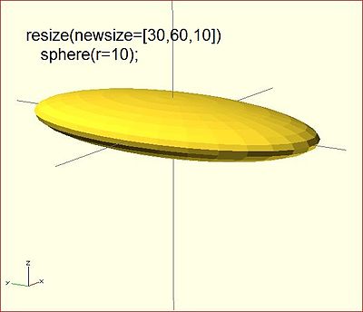
resize
Modifies the size of the child object to match the given x,y, and z.
resize() is a CGAL operation, and like others such as render() operates with full geometry, so even in preview this takes time to process.
Usage Example:
// resize the sphere to extend 30 in x, 60 in y, and 10 in the z directions.
resize(newsize=[30,60,10]) sphere(r=10);
If x,y, or z is 0 then that dimension is left as-is.
// resize the 1x1x1 cube to 2x2x1
resize([2,2,0]) cube();
If the 'auto' parameter is set to true, it auto-scales any 0-dimensions to match. For example.
// resize the 1x2x0.5 cube to 7x14x3.5
resize([7,0,0], auto=true) cube([1,2,0.5]);
The 'auto' parameter can also be used if you only wish to auto-scale a single dimension, and leave the other as-is.
// resize to 10x8x1. Note that the z dimension is left alone.
resize([10,0,0], auto=[true,true,false]) cube([5,4,1]);
rotate
Rotates its child 'a' degrees about the axis of the coordinate system or around an arbitrary axis. The argument names are optional if the arguments are given in the same order as specified.
//Usage:
rotate(a = deg_a, v = [x, y, z]) { ... }
// or
rotate(deg_a, [x, y, z]) { ... }
rotate(a = [deg_x, deg_y, deg_z]) { ... }
rotate([deg_x, deg_y, deg_z]) { ... }
The 'a' argument (deg_a) can be an array, as expressed in the later usage above; when deg_a is an array, the 'v' argument is ignored. Where 'a' specifies multiple axes then the rotation is applied in the following order: x, y, z. That means the code:
rotate(a=[ax,ay,az]) {...}
is equivalent to:
rotate(a=[0,0,az]) rotate(a=[0,ay,0]) rotate(a=[ax,0,0]) {...}
The optional argument 'v' is a vector and allows you to set an arbitrary axis about which the object is rotated.
For example, to flip an object upside-down, you can rotate your object 180 degrees around the 'y' axis.
rotate(a=[0,180,0]) { ... }
This is frequently simplified to
rotate([0,180,0]) { ... }
When specifying a single axis the 'v' argument allows you to specify which axis is the basis for rotation. For example, the equivalent to the above, to rotate just around y
rotate(a=180, v=[0,1,0]) { ... }
When specifying a single axis, 'v' is a vector defining an arbitrary axis for rotation; this is different from the multiple axis above. For example, rotate your object 45 degrees around the axis defined by the vector [1,1,0],
rotate(a=45, v=[1,1,0]) { ... }
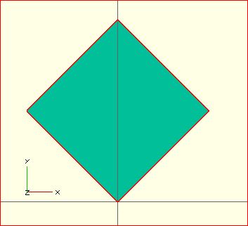
Rotate with a single scalar argument rotates around the Z axis. This is useful in 2D contexts where that is the only axis for rotation. For example:
rotate(45) square(10);
Rotation rule help

For the case of:
rotate([a, b, c]) { ... };
"a" is a rotation about the X axis, from the +Y axis, toward the +Z axis.
"b" is a rotation about the Y axis, from the +Z axis, toward the +X axis.
"c" is a rotation about the Z axis, from the +X axis, toward the +Y axis.
These are all cases of the Right Hand Rule. Point your right thumb along the positive axis, your fingers show the direction of rotation.
Thus if "a" is fixed to zero, and "b" and "c" are manipulated appropriately, this is the spherical coordinate system.
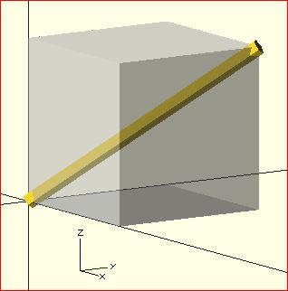
So, to construct a cylinder from the origin to some other point (x,y,z):
x= 10; y = 10; z = 10; // point coordinates of end of cylinder

length = norm([x,y,z]);  // radial distance
b = acos(z/length); // inclination angle
c = atan2(y,x);     // azimuthal angle

rotate([0, b, c])
    cylinder(h=length, r=0.5);
%cube([x,y,z]); // corner of cube should coincide with end of cylinder
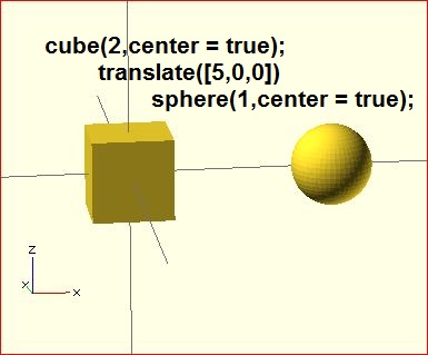
translate
Translates (moves) its child elements along the specified vector. The argument name is optional.
Example:
translate(v = [x, y, z]) { ... }
cube(2,center = true);
translate([5,0,0])
   sphere(1,center = true);
mirror
Mirrors the child element on a plane through the origin. The argument to mirror() is the normal vector of a plane intersecting the origin through which to mirror the object.
Function signature:
mirror(v= [x, y, z] ) { ... }
Examples
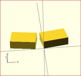
The original is on the right side. Note that mirror doesn't make a copy. Like rotate and scale, it changes the object.
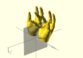
hand(); // originalmirror([1,0,0]) hand();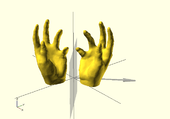
hand(); // originalmirror([1,1,0]) hand();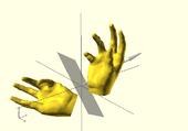
hand(); // originalmirror([1,1,1]) hand();
rotate([0,0,10]) cube([3,2,1]);
mirror([1,0,0]) translate([1,0,0]) rotate([0,0,10]) cube([3,2,1]);
multmatrix
Multiplies the geometry of all child elements with the given affine transformation matrix, where the matrix is 4×3 - a vector of 3 row vectors with 4 elements each, or a 4×4 matrix with the 4th row always forced to [0,0,0,1].
Usage: multmatrix(m = [...]) { ... }
This is a breakdown of what you can do with the independent elements in the matrix (for the first three rows):
| [Scale X] | [Shear X along Y] | [Shear X along Z] | [Translate X] |
| [Shear Y along X] | [Scale Y] | [Shear Y along Z] | [Translate Y] |
| [Shear Z along X] | [Shear Z along Y] | [Scale Z] | [Translate Z] |
The fourth row is forced to [0,0,0,1] and can be omitted unless you are combining matrices before passing to multmatrix, as it is not processed in OpenSCAD. Each matrix operates on the points of the given geometry as if each vertex is a 4 element vector consisting of a 3D vector with an implicit 1 as its 4th element, such as v=[x, y, z, 1]. The role of the implicit fourth row of m is to preserve the implicit 1 in the 4th element of the vectors, permitting the translations to work. The operation of multmatrix therefore performs m*v for each vertex v. Any elements (other than the 4th row) not specified in m are treated as zeros.
This example rotates by 45 degrees in the XY plane and translates by [10,20,30], i.e. the same as translate([10,20,30]) rotate([0,0,45]) would do.
angle=45;
multmatrix(m = [ [cos(angle), -sin(angle), 0, 10],
                 [sin(angle),  cos(angle), 0, 20],
                 [         0,           0, 1, 30],
                 [         0,           0, 0,  1]
              ]) union() {
   cylinder(r=10.0,h=10,center=false);
   cube(size=[10,10,10],center=false);
}
The following example demonstrates combining affine transformation matrices by matrix multiplication, producing in the final version a transformation equivalent to rotate([0, -35, 0]) translate([40, 0, 0]) Obj();. Note that the signs on the sin function appear to be in a different order than the above example, because the positive one must be ordered as x into y, y into z, z into x for the rotation angles to correspond to rotation about the other axis in a right-handed coordinate system.
y_ang=-35;
mrot_y = [ [ cos(y_ang), 0,  sin(y_ang), 0],
           [         0,  1,           0, 0],
           [-sin(y_ang), 0,  cos(y_ang), 0],
           [         0,  0,           0, 1]
         ];
mtrans_x = [ [1, 0, 0, 40],
             [0, 1, 0,  0],
             [0, 0, 1,  0],
             [0, 0, 0,  1]
           ];
module Obj() {
   cylinder(r=10.0,h=10,center=false);
   cube(size=[10,10,10],center=false);
}

echo(mrot_y*mtrans_x);
Obj();
multmatrix(mtrans_x) Obj();
multmatrix(mrot_y * mtrans_x) Obj();
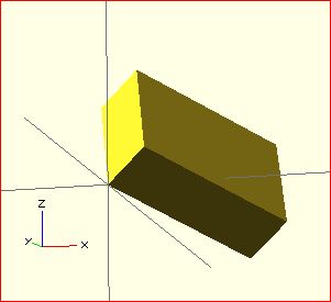
This example skews a model, which is not possible with the other transformations.
M = [ [ 1  , 0  , 0  , 0   ],
      [ 0  , 1  , 0.7, 0   ],  // The "0.7" is the skew value; pushed along the y axis as z changes.
      [ 0  , 0  , 1  , 0   ],
      [ 0  , 0  , 0  , 1   ] ] ;
multmatrix(M) {  union() {
    cylinder(r=10.0,h=10,center=false);
    cube(size=[10,10,10],center=false);
} }
More?
Learn more about it here:
color
Displays the child elements using the specified RGB color + alpha value. This is only used for the F5 preview as CGAL and STL (F6) do not currently support color. The alpha value defaults to 1.0 (opaque) if not specified.
Function signature:
color( c = [r, g, b, a] ) { ... }
color( c = [r, g, b], alpha = 1.0 ) { ... }
color( "#hexvalue" ) { ... }
color( "colorname", 1.0 ) { ... }
Note that the r, g, b, a values are limited to floating point values in the range [0,1] rather than the more traditional integers { 0 ... 255 }. However, nothing prevents you to using R, G, B values from {0 ... 255} with appropriate scaling: color([ R/255, G/255, B/255 ]) { ... }
[Note: Requires version 2011.12]
Colors can also be defined by name (case insensitive). For example, to create a red sphere, you can write color("red") sphere(5);. Alpha is specified as an extra parameter for named colors: color("Blue",0.5) cube(5);
[Note: Requires version 2019.05]
Hex values can be given in 4 formats, #rgb, #rgba, #rrggbb and #rrggbbaa. If the alpha value is given in both the hex value and as separate alpha parameter, the alpha parameter takes precedence.
The available color names are taken from the World Wide Web consortium's SVG color list. A chart of the color names is as follows,
(note that both spellings of grey/gray including slategrey/slategray etc are valid):
|
|
|
|
| |||||||||||||||||||||||||||||||||||||||||||||||||||||||||||||||||||||||||||||||||||||||||||||||||||||||||||||||||||||||||||||||||||||||||||||||||||||||||
Example
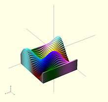
Here's a code fragment that draws a wavy multicolor object
  for(i=[0:36]) {
    for(j=[0:36]) {
      color( [0.5+sin(10*i)/2, 0.5+sin(10*j)/2, 0.5+sin(10*(i+j))/2] )
      translate( [i, j, 0] )
      cube( size = [1, 1, 11+10*cos(10*i)*sin(10*j)] );
    }
  }
↗ Being that -1<=sin(x)<=1 then 0<=(1/2 + sin(x)/2)<=1 , allowing for the RGB components assigned to color to remain within the [0,1] interval.
Chart based on "Web Colors" from Wikipedia
Example 2
In cases where you want to optionally set a color based on a parameter you can use the following trick:
 module myModule(withColors=false) {
    c=withColors?"red":undef;
    color(c) circle(r=10);
 }
Setting the colorname to undef keeps the default colors.
offset
[Note: Requires version 2015.03]
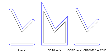
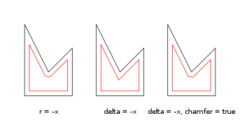
Offset generates a new 2d interior or exterior outline from an existing outline. There are two modes of operation. radial and offset. The offset method creates a new outline whose sides are a fixed distance outer (delta > 0) or inner (delta < 0) from the original outline. The radial method creates a new outline as if a circle of some radius is rotated around the exterior (r>0) or interior (r<0) original outline.
The construction methods can either produce an outline that is interior or exterior to the original outline. For exterior outlines the corners can be given an optional chamfer.
Offset is useful for making thin walls by subtracting a negative-offset construction from the original, or the original from a Positive offset construction.
Offset can be used to simulate some common solid modeling operations:
- Fillet: offset(r=-3) offset(delta=+3) rounds all inside (concave) corners, and leaves flat walls unchanged. However, holes less than 2*r in diameter vanish.
- Round: offset(r=+3) offset(delta=-3) rounds all outside (convex) corners, and leaves flat walls unchanged. However, walls less than 2*r thick vanish.
- Parameters
- r
- Double. Amount to offset the polygon. When negative, the polygon is offset inward. R specifies the radius of the circle that is rotated about the outline, either inside or outside. This mode produces rounded corners.
- delta
- Double. Amount to offset the polygon. Delta specifies the distance of the new outline from the original outline, and therefore reproduces angled corners. When negative, the polygon is offset inward. No inward perimeter is generated in places where the perimeter would cross itself.
- chamfer
- Boolean. (default false) When using the delta parameter, this flag defines if edges should be chamfered (cut off with a straight line) or not (extended to their intersection).
Examples
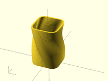
// Example 1

linear_extrude(height = 60, twist = 90, slices = 60) {
   difference() {
     offset(r = 10) {
      square(20, center = true);
     }
     offset(r = 8) {
       square(20, center = true);
     }
   }
 }
// Example 2

module fillet(r) {
   offset(r = -r) {
     offset(delta = r) {
       children();
     }
   }
}
minkowski
Displays the minkowski sum of child nodes.
Usage example:
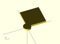
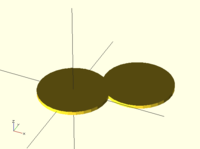
Say you have a flat box, and you want a rounded edge. There are multiple ways to do this (for example, see hull below), but minkowski is elegant. Take your box, and a cylinder:
 $fn=50;
 cube([10,10,1]);
 cylinder(r=2,h=1);
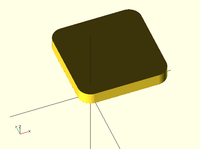
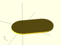
Then, do a minkowski sum of them (note that the outer dimensions of the box are now 10+2+2 = 14 units by 14 units by 2 units high as the heights of the objects are summed):
$fn=50;
minkowski()
{
  cube([10,10,1]);
  cylinder(r=2,h=1);
}
NB: The origin of the second object is used for the addition. If the second object is not centered, then the addition is asymmetric. The following minkowski sums are different: the first expands the original cube by 0.5 units in all directions, both positive and negative. The second expands it by +1 in each positive direction, but doesn't expand in the negative directions.
minkowski() {
    cube([10, 10, 1]);
    cylinder(1, center=true);
}
minkowski() {
    cube([10, 10, 1]);
    cylinder(1);
}
Warning: for high values of $fn the minkowski sum may end up consuming lots of CPU and memory, since it has to combine every child node of each element with all the nodes of each other element. So if for example $fn=100 and you combine two cylinders, then it does not just perform 200 operations as with two independent cylinders, but 100*100 = 10000 operations.
hull
Displays the convex hull of child nodes.
Usage example:
hull() {
    translate([15,10,0]) circle(10);
    circle(10);
}
The Hull of 2D objects uses their projections (shadows) on the xy plane, and produces a result on the xy plane. Their Z-height is not used in the operation.
Combining transformations
When combining transformations, it is a sequential process, but going right-to-left. That is
rotate( ... ) translate ( ... ) cube(5) ;
would first move the cube, and then move it in an arc (while also rotating it by the same angle) at the radius given by the translation.
translate ( ... ) rotate( ... ) cube(5) ;
would first rotate the cube and then move it to the offset defined by the translate.
color("red")   translate([0,10,0])  rotate([45,0,0])     cube(5);
color("green") rotate([45,0,0])     translate([0,10,0])  cube(5);